A Demonstration of the Asphalt Pavement Scanner

This guest post was written by Chuck Oden, PhD of ESS. This white paper was originally published by ESS and we are sharing it here, with his permission.

Introduction

The Humboldt Asphalt Pavement Scanner (APS) is a revolutionary new system that provides detailed and comprehensive quality information for new asphalt mats without the use of nuclear sources. To demonstrate these capabilities, a short survey was made at a new subdivision under construction. This report demonstrates the richness of the APS data and examines how the APS system can be used for process control during construction and for inspection and acceptance after construction.

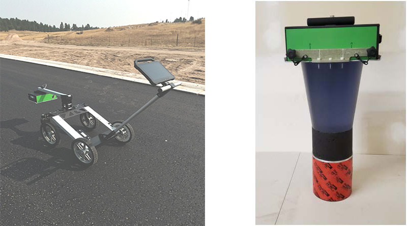
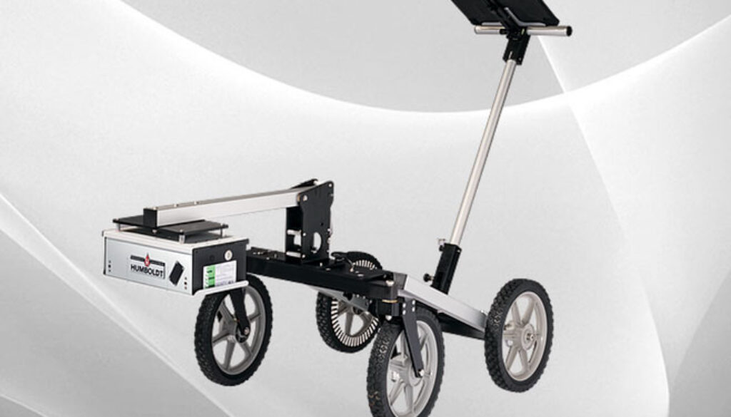
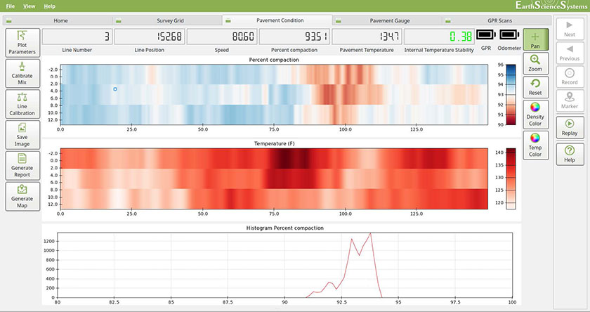
The APS system has three configurations that can be used to generate compaction maps, make gauge measurements, and create mix calibrations. These configurations are shown in Figure 1 and described below. The entire system has been designed for ease of use without troublesome cables or connectors. Figure 2 shows a software screenshot where compaction, surface temperature, and a compaction histogram are shown on a tablet computer. 

An Example Survey

Two surveys were conducted at a new residential subdivision where two SuperPave lifts (mats) with a nominal thickness of 2 inches were placed directly over a compacted subgrade. The streets were paved using a screed that was one lane wide with a hot center joint between the lanes. The first survey was conducted after the base lift was installed just after the roller compactor stage was completed, and a second survey was conducted a few hours after the top lift was installed. The APS was setup in cart configuration and each lane of the two-lane road was surveyed using three 150 foot long survey lines. Each survey line was offset by about 5 feet from the previous line to provide three lines for each lane. In cart mode the APS system scans a surface area with a diameter of 2 feet and a depth of 1.5 or 3 inches (user selectable). An additional survey line was taken with the cart straddling the center joint. APS cart surveys are conducted at walking speeds and surveys can keep pace with the roller compactors. The pavement surface must be dry when taking APS measurements.

The scan head for the APS system contains a high accuracy GPS unit so that the measurements can be mapped as shown in Figure 3 which shows measurements from the top lift. The depth of investigation was 1.5 inches and the red coloring indicates areas where the compaction is less than 92%. The road outlines were obtained from county assessor maps because the new subdivision does not yet appear on other map services such as Google maps. It is clear that the APS survey results provide a much better indication of the uniformity and quality of the installation than results from a few cores or density gauge readings. With only a few cores or gauge readings, one or two low compaction readings could cast the quality of the entire job in a bad light. On the other side of the coin, with only a few spot readings there could be large swaths of improperly compacted asphalt that remain undetected. As might be expected, the compaction levels along the center joint are lower than in the middle of each lane. It is also clear that sometimes the compaction on one side of the road is different than on the other side, and on this job the results indicate that there are significant areas that were insufficiently compacted. Incorporating the APS system into the construction process would allow workers to address the under compacted regions before the mat cooled to the point where it can no longer be compacted.

Figure 2 shows an example of the real-time display of compaction and surface temperature measurements where three survey lines are shown as three color bands. The real-time plots only use odometer data, and mapped images such as those shown in Figure 3 can be produced using the tablet computer after the survey is complete using both odometer and GPS data. The survey data in Figure 3 was collected with an independent GPS receiver which typically provides a positional accuracy of 3-6 feet. An RTK GPS system is also available for the APS system that provides a positional accuracy of about ½ inch.

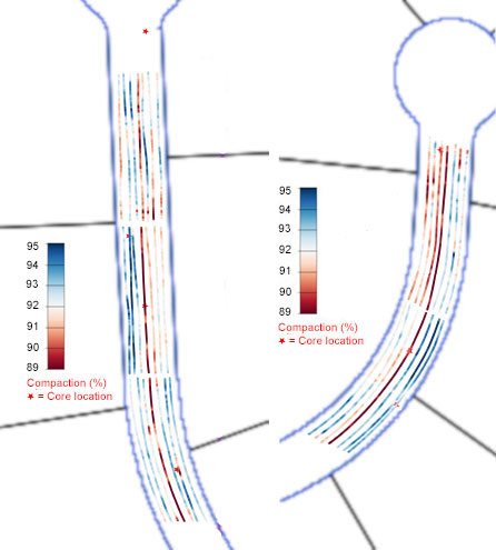
In order to provide compaction readings, the APS system uses mix calibrations to convert dielectric constant to compaction. This calibration is different for each mix design, and this calibration is analogous to determining maximum density to convert density readings into percent compaction. For this survey the mix calibration was obtained from cores that were collected a few days after construction (core locations are shown in Figure 3). The calibration section of this paper discusses various calibration methods for the APS system.

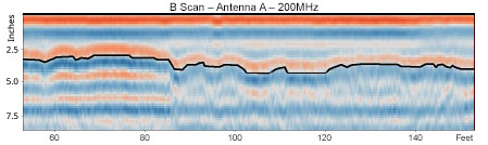
Other measurements provided by the APS system include surface temperature, surface roughness, and thickness. The surface temperature can be used to indicate when the pavement is too cold for further compaction. Temperature anomalies can indicate changes in mix uniformity such as segregation, a cold section of the mix, or they may simply indicate a region of the mat that was shaded from the sun by a construction vehicle. Maps generated using GPS data such as those shown in Figure 3 can be produced using surface temperature or roughness measurements. Finally, the GPR B-scans can be used to indicate the thickness of the mat (see Figure 4).

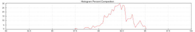
The APS software can generate reports that contain statistics of the measurements. Pass/fail metrics can be established for compaction and statistics for under compaction, proper compaction, and over compaction can be reported. Figure 5 below shows a histogram of compaction. This information provides an overall indication of the quality and consistency of the job that cannot be obtained from a small number of density gauge measurements or cores.

Mix Calibration

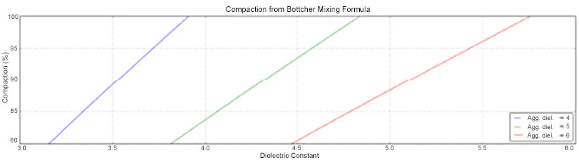
Traditional nuclear density gauges use the maximum density of an asphalt mix to convert from density to compaction. Similarly, dielectric measurements of asphalt concrete can be converted to compaction using the dielectric constant of the aggregate. The dielectric constant of granitic material is usually in the range of 4 to 5, while that of limestone is typically closer to 6. Figure 7 below shows the theoretical relationship between the dielectric constant of the mix and compaction for different aggregate dielectrics using the Bottcher mixing formula (Leng, 2011, see Appendix I). Theoretical mixing formulas are useful for investigating cause and effect, but in practice mix calibrations are determined by fitting an exponential curve to calibration data. These data are a set of measured dielectric and independently measured compaction values. The exponential relationship that relates dielectric constant to compaction is given below,

C=a⋅e^b⋅ϵ_ac

where C is compaction, a and b are fitting constants and εac is the dielectric constant of the asphalt concrete. It is beneficial to use a set of calibration measurements that span the expected compaction values rather than
lying near the center of the expected range
so that extrapolation is avoided.

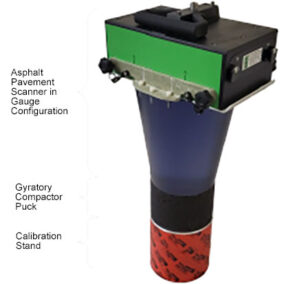
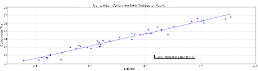
The APS system offers three mix calibration methods: 1) using gyratory compactor pucks, 2) using cores, or 3) using nuclear gauge readings. The compactor puck method is the most accurate and is recommended. Figure 8 shows the APS system configured for measuring gyratory compactor pucks, and Figure 9 below shows a mix calibration curve generated by taking compactor puck measurements. Since compactor pucks are created before construction during the mix design phase, puck measurements can be made to obtain a mix calibration so that calibrated compaction readings can be made during construction. This allows construction crews to obtain compaction information during construction so that rolling patterns can be changed or under compacted areas can be addressed. The APS system measures the dielectric constant of gyratory pucks by measuring the time-of-flight of a radar wave through the puck, and therefore the total volume of the puck is measured with both the APS system and the independent weight – volume measurements. This APS measurement also requires a precise puck thickness measurement which can be a source of error if performed carelessly.

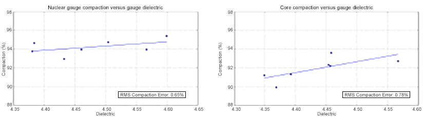
It is also possible to create a mix calibration from nuclear gauge readings or from cores taken at the construction site. The disadvantage of these methods is that the volume of investigation of the nuclear gauge, core, and APS gauge readings is different, which can lead to discrepancies between the measurements. The APS gauge reads to a depth of about 2.5 inches (6 cm) with a diameter of about 12 inches (30 cm). Nuclear gauges typically measure to depths of 1 – 4 inches (2.5 – 10 cm) with similar diameters. Cores typically have a diameter of 4 or 6 inches (10 or 15 cm) and the thickness can be more than the gauge investigation depths. Subsequently the deviation of the calibration reference points from mix calibrations (blue line in Figures 9 and 10) can be substantial.

Figure 10 below shows calibrations obtained from APS gauge versus nuclear gauge readings, and from APS gauge versus cores for the survey presented above. Figures 9 and 10 show that the RMS error of the measured compaction values from the calibration curve is more (0.65% and 0.78% for gauge and cores respectively) than that for the gyratory puck calibration (0.3%). The variability of nuclear gauge readings is typically too large for use as a calibration standard for the APS system (see Appendix II). It is noteworthy that the APS gauge measurements are extremely repeatable (in contrast to nuclear gauge readings). For example the standard deviation of 26 repeated dielectric measurements was 0.005, which corresponds to about 0.1% compaction (by comparison, the standard deviation of one-minute nuclear gauge measurements is typically ~2%; Stroup-Gardiner and Newcomb, 1988). For the case of the survey presented above, another source of discrepancy is that several sets of multiple markings were placed on the pavement in close proximity at each core/gauge measurement location. The cores were collected days after the APS survey and confusion with the markings could have caused the core locations to be as much as foot from the location of the APS gauge measurements.

Instrument Calibration

Using the dielectric constant to indicate compaction requires a precision instrument that provides accurate and repeatable measurements. The APS system has been factory calibrated and only periodic background measurements need to be taken while conducting field operations to maintain calibration. To assure users that the APS instrument is operating properly, a reference dielectric puck is available so that the performance of the unit can be verified in the field at any time.

Conclusions

The Humboldt Asphalt Pavement Scanner is a groundbreaking new system that provides unprecedented detail in Q/A and Q/C inspections of new asphalt construction. Surveys can be made continuously at walking speed that keep pace with paving operations. The system has been designed to dovetail into existing workflows from the design phase, to the construction phase, and finishing with the inspection phase. These capabilities are provided by two system configurations: the cart mode and the puck calibration mode.

Contractors can use increased coverage of the APS system to reduce risk and assure their customers that they are providing a quality product. During construction the locations of under compacted zones can be identified while the mat is still warm enough for further compaction. Compaction maps allow contractors to better assess their risk from random inspections from DOTs and owners. Finally, the detailed mapping and reporting abilities provides DOTs and owners assurance that they are receiving a uniform and quality product.

Appendix I: Bottcher Mixing Formula

With theoretical mixing formulas, one can calculate the expected dielectric constant of a mixture from the volume fractions and dielectric constant of the constituents (i.e., aggregate, binder, and air). The Bottcher mixing formula is given below, 

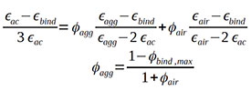
where ε_ac, ε_bind, ε_agg, and ε_air are the dielectric constant of asphalt concrete, binder, aggregate, and air respectively, and φ_agg, φ_air, are the volume fraction of aggregate, and air respectively, and φ_bind,max is the volume fraction of binder at maximum compaction.

Appendix II: Variability of Nuclear Gauge Readings

When taking nuclear gauge readings on a mat, the Colorado Department of Transportation requires four measurements: two repeat measurements with the gauge on one orientation (i.e., right orientation), and two more readings with the gauge at the same location be turned 180 degrees (i.e., left orientation). ESS conducted a survey in a newly paved parking lot where nuclear gauge readings were taken at 25 different locations, with some locations in the middle of the lot and some near the edges. The standard deviation between the left and right readings at each location was 2.1% compaction. The offset in the sensor locations in the nuclear gauge (Instrotek model 3500 Explorer) was about 30 cm (12 inches) between the left and right orientations. In another study, the Wisconsin Department of Transportation (Schmitt, 2006) compared densities obtained from cores to nuclear gauge readings at 128 different locations on 16 different paving projects and found that the difference standard deviation between compaction readings from the two methods was 1.5%. The conclusion is that the variability in nuclear gauge readings is too high to use as a calibration standard for the APS system.